Sounds of STEREO
Play movie: demo2.mpg (19 MB)
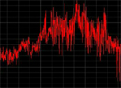
Using the UC Berkeley church bells as the basic element of this sonification, we sonify the solar wind density from July 7, 2007. Solar wind density is the number of mostly hydrogen ions, which are protons, in a given volume (cubic centimeter in this case). Time is on the x-axis of this movie, spanning 24 hours. The y-axis is the solar wind density from 0.44 cm-3 to 6.86 cm-3. At low solar wind density, four bells play together. The higher the wind density, the more the four bells will play to the "beat of their own drum" (i.e. own tempi). The data is also sonified such that the lower the solar wind density is, the less dissonance and the higher the solar wind density is, the higher dissonance the sound is. Because 2007 had very few solar storms, the wind was pretty mild and the contrast in the maximum wind and minimum wind is not as large as one might think. To hear the contrast more clearly in the low and high density solar wind, please listen to and watch the following movies.
pulse.mpg (4.9MB) drone.mpg (3.9MB) both.mpg (6.9MB)
This first movie demonstrates the sonification at the first solar wind density value (~0.5 cm-3), playing that value as a constant solar wind density until it moves to the top density value (~ 6.5 cm-3). With this contrast, it becomes clearer how there are more bell sounds at higher density solar winds.
The second movie demonstrates the second sonification of this data. Again the bells are used but now dissonance in the bells is used. The lower the solar wind density is, the less dissonance and the higher the solar wind density is, the higher dissonance the sound is. High dissonance is often used in music in Western movies to indicate terror, violence and such, on the screen. We have used this sonification since solar storms with increases in solar wind density can cause electrical blackouts in cities, damage satellites and spacecraft, and harm unprotected astronauts.
The last movie demonstrates both sonifications played together during the lowest and highest solar wind values.
Spectrograph
Click on the image to watch the sonification of each data point shwon in color:
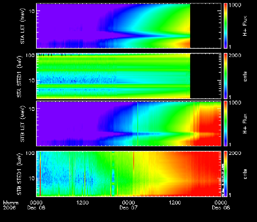
Above image shows and plays the flux of high energy (1-10MeV) ions in the solar wind as a Coronal Mass Ejection (CME) travels by the STEREO satellites. The sound on the left and right speakers are coming from the left and right images which are from STEREO A and B sattelites respectively. This event occured on December 6th, 2006 and we are showing 40 hours of the data. The flux is larger when the sound is more complex and when the color on the images is on the red side of the rainbow colors (yellow, orange, red). These sounds come from running a plot of the flux of particles through the IMPACT sonification "Stereo Spectro" software application. To see the original data, see below. To hear the sound without the animation, click here (mp3, 5.1MB).
Full Data
Click to enlarge