Astronomy 10: Lecture 13
Lecture 13
Wednesday, June 19th 2002. Reading: Cosmic Perspective Chapter 15
Stars and their Properties
Distance
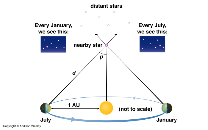 Use trigonometric parallax (triangulation) for nearby stars.
Parallax = angle subtended (i.e., covered) by 1 A.U., the distance from Earth to the Sun. (1/2 of the diameter of Earth's orbit).
As distance increases the parallax angle decreases. Ultimately limited by the smallest angles measurable (resolved). The atmosphere limits resolution ability, must go to space --> Hipparcos satellite.
The distance at which 1 A.U. subtends 1" (one arc second) is called 1 parsec (pc). (parallax arc second).
dpc = 1/p(")
1 pc = 3.26 Light-years. Distance to nearest star, Alpha-Centauri:
p = 0.762" ---> d = 1.31 pc = 4.27 light-years
Best angle measurements of Hipparcos were down to p = 0.002" ---> d = 500 pc (1,630 light-years).
|
Space Motion
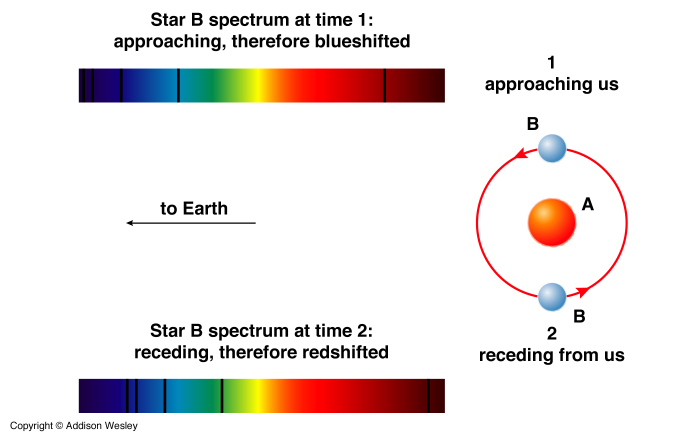
- Radial Velocity: the component of velocity along our line of sight (perpendicular to the plane of the sky). We measure this by the doppler shift of spectral lines in the spectra of the stars.

 /0 = v/c
< 0 --> Blueshift: moving toward us
> 0 --> Redshift: moving away from us
- Proper Motion: the apparent motion of a star through the sky due to its Transverse velocity, vT, which is the component of a star's total space velocity across our line of sight.
measured as an angular speed (typically 0.1"/yr for nearby stars), but to convert to physical speed (km/s) need to know the distance
vT = 4.74 ("/yr)dpc
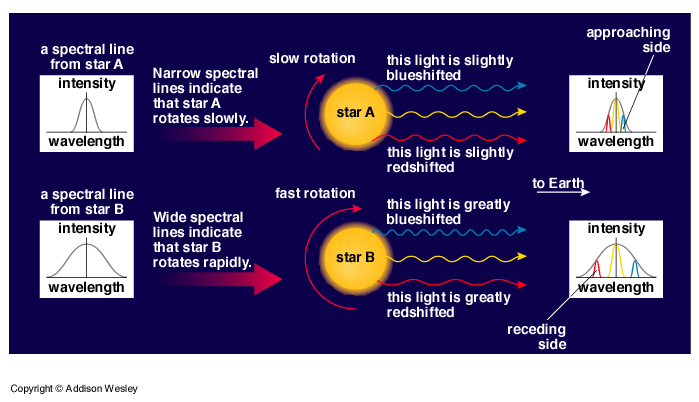
- Spin: If a star is spinning (and they all seem to be) then, as it spins, one side of it is moving toward us while the other side is moving away from us. This will cause the width of spectral lines from its surface to be Broadened due to the doppler shift. The width of their broadening is and so gives us the rate of spin of the star.
Mass and Size
Direct measurements of mass and size of stars are not possible with our current Earth-bound technology. But we can infer these quantities with knowledge of physics and geometry if the stars are members of a binary system.
- Binary Systems: Over 50% of the stars in the sky are actually multiple systems bound together by mutual gravity. Most are double. Some are visual binary systems: they can be seen in a telescope as two stars. Others are spectroscopic binary systems: only one star can be seen but the spectra is that of two stars that shifts back and forth from doppler effect. The two stars are in orbit about one another.
- Kepler's 3rd Law: applies not only to planets in orbit around stars, but stars in orbit around a common center of mass. In binary systems we can measure the period of their orbits, and if we observe them carefully we can also get the size of their orbits (semimajor axis) by measuring their proper motion and parallax. Thus using Netwon's form of Kepler's third law we can measure the sum of their masses.
P2 = 4 2/G(m1+m2) * a3
- Center of Mass: In order to get the individual masses of the stars we can make even more careful measurements of the binary orbit and determine each star's distance to their common center of mass. There is a simple relation between their distances from the center of mass and their masses:
m1a1 = m2a2
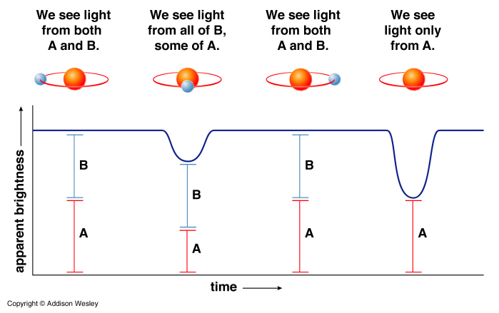
- Eclipsing binaries: Sometimes there is an extraordinary alignment of a binary system to our line of sight and the two stars eclipse one another. When this happens the combined light from the two stars changes as one star passes in front of the other. There appear dips in the light curve. We can measure the stars' orbital velocities using the doppler shift of light and then use the timing of the eclipses to infer the size of each star.
(d = vt)
Temperature
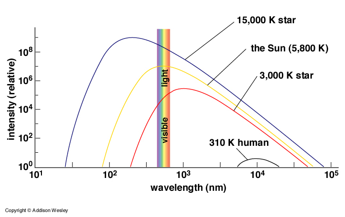
We can measure the temperature of the surface (photosphere) of stars by using their color. When we examine their energy spectrum we can see that they are thermal emitters. Thus, we can can fit the mathematical spectrum of a theoretical thermal emitter over the observed spectrum and infer the effective surface temperature of the star using Wien's Law:
peakT = 2.898x10⁻³ m*K
We can also infer the temperature of the surface from the specific spectral lines that are seen. Recall that spectral lines arise from transitions of an electron from one level to another in an atom. The electron may only emit or absorb very specific wavelengths of light for specific transitions. So, for example, say we see an absorption line of hydrogen which indicates that an electron has absorbed a photon and jumped from level 4 to level 7 in the atom. For the electron to already be excited enough to be in level 4 the atoms in the star's surface must be moving fast and hitting each other very often. This kind of motion is in fact how we define temperature. So this would be a pretty hot star.
Luminosity
Luminosity is the total amount of energy that leaves a star per unit time. It therefore has units of energy per time. Watts is one such unit (joules/s). ergs/s is another.
Stefan-Boltzmann Law: Recall that we had a relationship between the temperature of a thermal emitter and how much energy per unit surface area per unit time it emitted.
 =
=  T4
T4
So if we want to know how much total energy per second a thermal emitter emits we need to multiply by its total surface area. Stars are spherical, so SA = 4R2. Thus the luminosity, L, of a star is related to its radius, R, and surface temperature, T.
L = 4R2T4
Inverse Square Law of Light:
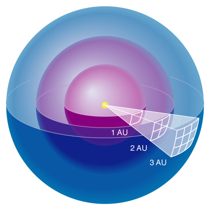 When you observe a star from a distance, d, you do not directly observe its luminosity because you only intercept a small fraction of the energy that left its surface. You observe the star's brightness, b. Brightness has unit of energy per unit surface area detected per unit time. Since light spreads away from a star in a spherical shell you can see that the amount of energy per unit surface area per unit time observed at a distance is just the Luminosity of the star divided by the surface area of a shell at the distance of the observer. This gives us the inverse square law of light.
b = L/(4d2)
When you observe a star from a distance, d, you do not directly observe its luminosity because you only intercept a small fraction of the energy that left its surface. You observe the star's brightness, b. Brightness has unit of energy per unit surface area detected per unit time. Since light spreads away from a star in a spherical shell you can see that the amount of energy per unit surface area per unit time observed at a distance is just the Luminosity of the star divided by the surface area of a shell at the distance of the observer. This gives us the inverse square law of light.
b = L/(4d2)
This says that if you move twice as far from a star (from some starting position) the star will become 4 times as dim.
It also says that if you know the distance to a star, and you measure its brightness, you can infer its luminosity. Then you can measure its temperature from spectrum and hence get its size.
|
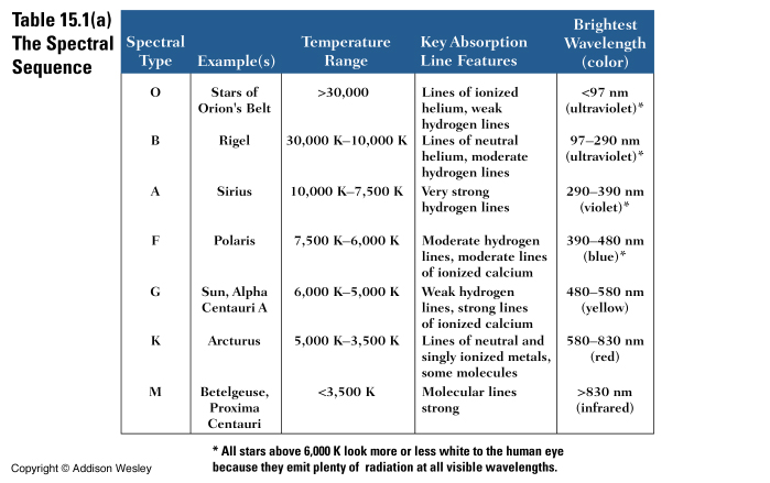
Spectral Classes
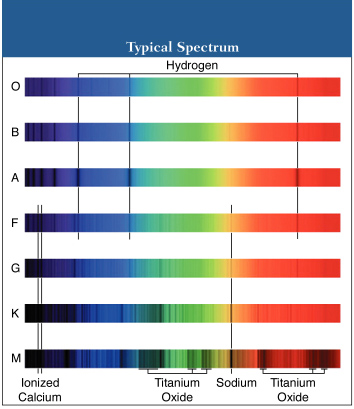 The spectra of stars are varied, but there are trends. In the early part of the 20th century a classification scheme was devised for stars based on their spectra. The scheme originally was based only on the relative strengths of Hydrogen lines in the stars' atmosphere. Type A stars have strongest hydrogen lines, type O the weakest.
The different classes were then later arranged in order of decreasing surface temperature (some where rejected due to redundancy). From hottest to coolest the order is:
O B A F G K M (L)
The mnemonic most commonly used to remember this sequence is
"Oh Be A Fine Girl/Guy Kiss Me (Lovingly)"
Make up your own and email it to me!
Old Baboons Angrily Fling Green Kiwis, Mangos, and Limes
|
A Summary of Stellar Properties
| Property | How it is determined |
| Brightness | directly measured |
| Color | -Compare brightness in two different E&M spectrum bands.
-Examine spectra of star |
| Temperature | Use color or spectra |
| Distance | -Directly measured via parallax
-Indirectly measured via method of standard candles |
| Luminosity | -use brightness and distance
-Eclipsing Binary: Use Temperature and Size |
| Radial Velocity | Doppler shift of spectral lines |
| Transverse Velocity | proper motion and distance |
| Rate of Spin | Doppler broadening of Spectral Lines |
| Size | -Luminosity and Temperature
-directly measure in an Eclipsing Binary |
| Mass | -Use Kepler's 3rd Law in Binary System.
-Infer from Luminosity and Temperature.
-Infer from spectral lines. |
| Chemical Composition | Spectral Lines |
| Strenth of Magnetic Field | Spectral Lines |
| Age | Main-Sequence Turn-off Point in a cluster
|
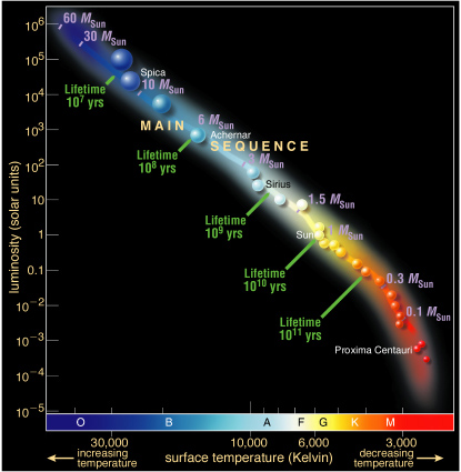
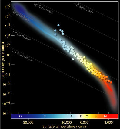
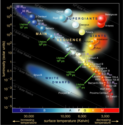
Hertzsprung-Russell Diagram
We are able to measure some critical physical properties stars. That's a first step in science: empirical observation.
Now we'd like to understand what it all means. We need to examine the raw data in some meaningful way to see if any patterns emerge. Then we'll be able to make hypotheses and test them out with further observations.
Radius Trend
In the regions above and below the Main Sequence there are other regions where stars seem to gather on the H-R diagram. On the upper right there are stars that are very luminous and have cool surfaces (hence they are red). In the lower left of the plot there are stars which are "white-hot" but much less luminous than the stars on the Main Sequence.
This leads us to consider what is different about these stars such that they have the same surface temperatures as stars on the main sequence but have different luminosities. The answer comes from the Stefan-Boltzmann Law:
L = 4R2T4
If two stars have the same temperature but different luminosities then they must have different radii. Stars with higher luminosity must therefore be bigger than stars with lower luminosities but the same temperature.
Hence, we call the stars in the upper right Red Giants and the stars in the lower left White Dwarfs.
Further analysis also finds that stars tend to have larger radii on the hotter (blue) end of the main sequence and smaller radii on the cooler (red) end of the main sequence.
Mass and Luminosity Trends
When we combine the information about mass that we have learned from the careful study of binary stars, we find that there is another important trend in the H-R diagram. The more luminous main sequence stars are also more massive. Thus the O and B main sequence stars are more massive than our Sun (a G star) which is in turn more massive than a K main sequence star. There is a quantifiable relationship between these quantities.
L  M4
Luminosity is roughly proportional to the mass raised to the 4th power. The mass of the Sun is M
M4
Luminosity is roughly proportional to the mass raised to the 4th power. The mass of the Sun is M = 2 x 1030 kg.
This relationship is only true for Main Sequence stars. There are also trends with the red giants and white dwarfs but they are not as simple. Generally, more luminous Red Giants are more massive.
Lifetimes of Stars on the Main-Sequence
Stars on the Main-Sequence are burning hydrogen into helium within their cores. Eventually they run out of fuel to burn and begin to die. As they die they leave the Main Sequence.
The Sun has enough fuel to live on the Main Sequence for 10 Billion years. Stars with greater mass have more fuel to burn, but they also have much higer Luminosities; they have to in order to maintain hydrostatic equillibrium. A star with twice the mass of the Sun has a luminosity which is 16 times greater than the Sun. So despite having twice the mass to fuse it will use it up 16 times faster than the Sun. It's lifetime will therefore be 2/16 = 1/8th that of the Sun: Just over a Billion years. More massive stars live even shorter lives. A star with a mass 30 times the Sun's would live on the Main Sequence for only a few million years. This is a very short time in a Cosmic sense.
Stars with very low mass have such low luminosities that they may live for 10s - 100s of billions of years on the Main Sequence.
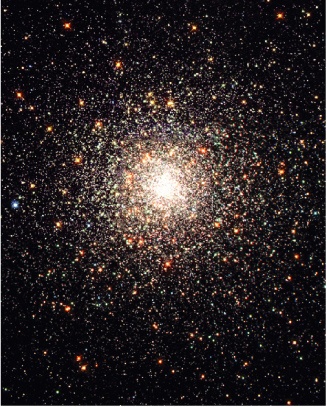
Clusters of Stars
 The H-R diagram of a cluster of Stars can be very instructive. Clusters contain stars which are all at the same distance from us. Thus differences in brightness translate directly into difference in Luminosity. This in fact is one way to measure distance, using the observed brightness of main-sequence stars in a cluster and comparing them to the known luminosities of similar main sequence stars in clusters with known distances.
The stars are also assumed to all be the same age. The theory of star formation would have that all the stars in the cluster formed from the same nebula that began to contract gravitationally.
There are two basic types of Clusters in the Galaxy: Open, which have several hundred widely spaced stars; and Globular, which have millions of stars all tightly packed into a glob.
|
 If we make an H-R diagram of a cluster and examine only the main sequence we would see that not all stars would be represented there. The top will likely be missing some stars. Where did they go?
They died, and left the main sequence. Since the high mass stars live the shortest lives they will be the first to shuffle off the mortal coil of the main sequence.
The main sequence will then peel away from top to bottom with time. And the point that it has peeled down to allows us to determine the age of the cluster. The stars at the top of the main sequence are just about to die and turn off the main sequence. So we call that point the turn off point.
Since we know what the lifetimes of stars in that location of the main sequence are then we know how old the cluster is.
|
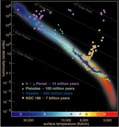 This is nicely illustrated by overplotting the Main Sequences of clusters of different ages.
Clusters with lots of hot blue stars are young. Clusters with yellow stars just turning off the main sequence are getting on in age. And those clusters with red stars turning off the main sequence are ancient.
Open clusters tend to be young, while globular clusters contain some of the oldest stars in the Universe.
|
Return to Class Notes Page
 HR-Diagram